Between 2009 and 2019, the U.S. vehicle market experienced a financial crisis, a federal scrappage program, record new vehicle sales, and a steady rise in average vehicle age. Yet through all of that change, the national vehicle scrappage rate remained relatively stable.
That stability is more interesting than it looks.
This article examines U.S. scrappage rate trends during that decade, the economic and policy forces behind them, and what those patterns reveal about fleet turnover, end-of-life vehicle dynamics, and long-term shifts in vehicle scrap value.
Key Takeaways
- U.S. scrappage rates moved within a relatively tight range from 2009 to 2019, but they still had meaningful peaks and dips (notably around 2013 and 2016).
- A stable scrappage rate does not automatically mean stable scrap payouts. Commodity prices, vehicle mix, and local market conditions matter more.
- If you’re pricing a scrap vehicle, the “rate” is background context. Your payout is driven by weight, metals, catalytic converter value, and where you’re selling.
Understanding the Scrappage Landscape
Let’s start with the basics, because the terms get mixed up all the time.
What Does “Scrappage Rate” Actually Mean?
A vehicle scrappage rate is the percentage of vehicles “in operation” that get retired from the active fleet in a given year. Think of it as the retirement rate for the whole national vehicle population.
It does not mean:
- The percentage of vehicles that go to a junkyard
- The percentage of vehicles that get crushed
- The percentage of vehicles that are “totaled” by insurance
It’s broader than that. It’s about vehicles leaving active use.
Why Industry People Track It
Scrappage is one of those quiet metrics that touches a lot of the automotive ecosystem:
Used Vehicle Supply
If fewer vehicles are scrapped, more older vehicles stay in circulation.
Parts and recycling
More scrappage can mean more salvageable parts and more metal feedstock.
Insurance and Repair
Scrappage trends are tied to repair decisions, total-loss thresholds, and consumer budgets.
Policy and Emissions
Governments watch fleet turnover because older vehicles tend to be less efficient and higher emitting.
A Quick Scale Check
Scrappage becomes more meaningful when viewed against the size of the U.S. vehicle fleet, which was often referenced at around 280 million vehicles by 2019. Applying a scrappage rate near 5% to a fleet of that size translates into millions of vehicles exiting active use each year, even if the percentage itself sounds modest.
That scale matters because it hints at something important: even small changes in scrappage rate can shift the supply of end-of-life vehicles by hundreds of thousands, sometimes millions, depending on fleet size.
U.S. scrappage rates (Cars, Light Trucks, All Light Vehicles), 2009–2019
From 2009 to 2019, U.S. vehicle scrappage rates moved within a relatively narrow range, but they did not remain flat. The longer-term average during 2000–2010 was about 5.3%, followed by a noticeable mid-decade decline.
Key reference points from the decade include
- 2013: scrappage rose to approximately 5.7%
- 2016: scrappage fell to about 4.4%, even as new vehicle sales peaked
- 2015–2019: scrappage stabilized around 4.5%
- 2019: approximately 5.1%
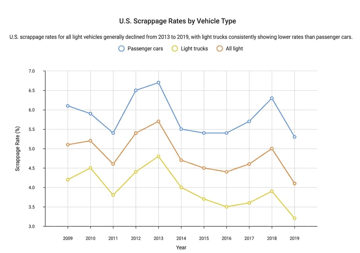
Scrappage Rates Over the Years
Year | Passenger cars | Light trucks | All light vehicles |
|---|---|---|---|
2009 | 6.1% | 4.2% | 5.1% |
2010 | 5.9% | 4.5% | 5.2% |
2011 | 5.4% | 3.8% | 4.6% |
2012 | 6.5% | 4.4% | 5.4% |
2013 | 6.7% | 4.8% | 5.7% |
2014 | 5.5% | 4.0% | 4.7% |
2015 | 5.4% | 3.7% | 4.5% |
2016 | 5.4% | 3.5% | 4.4% |
2017 | 5.7% | 3.6% | 4.6% |
2018 | 6.3% | 3.9% | 5.0% |
2019 | 5.3% | 3.2% | 4.1% |
Two observations stand out.
First, the rate fluctuated meaningfully within a relatively tight band rather than moving in dramatic swings. Second, the dip in 2016 occurred during peak new vehicle sales, which breaks from older assumptions that higher sales automatically lead to higher scrappage.
That divergence is central to understanding how fleet turnover actually behaved during this decade.
READ ALSO: Used Vehicle Market in the United States
The 2009 Shock: Cash for Clunkers and its Ripple Effects
The decade starts with a bang.
In 2009, the U.S. introduced the “Cash for Clunkers” program (CARS). The goal was to stimulate new vehicle sales and nudge people away from older, less fuel-efficient vehicles.
What happened, in plain terms
People traded in older cars and received a federal incentive, and those vehicles were permanently removed from the road. In total, approximately 677,081 vehicles were retired under the program.
That is not a small number but a huge one-time pulse of vehicles exiting the fleet.
Here’s the catch.
While the program succeeded in accelerating vehicle removals and temporarily boosting sales, research examining the 2009–2019 scrappage period shows that the long-term effects were more complex.
Analysts debated whether the program created lasting improvements in scrappage behavior or fuel economy. Some studies suggested that the long-term gains were limited, raising questions about whether the policy permanently changed fleet turnover patterns.
Why this matters for scrappage, not just sales
Cash for Clunkers also raised a bigger question.
If you remove a lot of older vehicles quickly, does that:
- Permanently change scrappage rates, or
- Simply shift scrappage timing, meaning vehicles that would have been scrapped later were scrapped sooner?
Economists refer to this concept as scrappage elasticity. In simple terms, it reflects how flexible vehicle owners are in deciding when to retire a car. If owners can extend a vehicle’s life through repairs, they may delay scrappage. If repair costs outweigh perceived value, retirement happens sooner.
In practice, owners are often more willing to keep vehicles running than policymakers assume. When budgets are tight or used vehicle prices are high, repairs become more attractive than replacement. That behavior can dampen the long-term impact of one-time scrappage incentives.
Why Scrappage Fell During Peak New Vehicle Sales
This is one of the most valuable insights because it goes against the simple old story.
A lot of people assume that more new sales equal more trade-ins, which equal more scrappage.
But in this decade, there was a point where that relationship didn’t behave normally.
2016: High Sales, Low Scrappage
In 2016, new car and light truck sales peaked at over 17 million units. During that same year, the scrappage rate fell to approximately 4.4%.
Historically, higher new vehicle sales were often associated with increased scrappage, as trade-ins and replacements moved older vehicles out of circulation. The 2016 divergence suggests a shift in that traditional pattern.
So why would that happen?
A few forces can push scrappage down even when sales are strong:
- 1.Vehicle longevity improved: Vehicles last longer now. Better engineering, better corrosion protection, better drivetrains, and better reliability.
- 2.Used vehicle prices and replacement math: If used vehicles are worth more, people delay scrapping. They sell, they keep, they fix. Scrapping becomes the last option.
- 3.Shift toward light trucks and SUVs: Growing demand for light trucks and SUVs complicated scrappage trends. This matters because scrappage behavior differs by vehicle type. Trucks can have different lifecycle patterns and can remain “useful” longer in many regions.
So even with strong sales, you can still see scrappage fall if the fleet is aging more slowly or people are simply hanging onto vehicles longer.
Factors influencing U.S. vehicle scrappage rates (2009–2019)
From 2009 to 2019, vehicle retirement patterns were shaped by economic conditions, fuel prices, policy decisions, consumer budgets, and improving vehicle durability. The rate may have looked steady on the surface, but the forces behind it were constantly shifting.
Understanding those forces helps explain why scrappage moved when it did and why it did not always track new vehicle sales. These factors are
Economic Conditions and Household Income
Regions with higher GDP per capita tend to have lower scrappage rates because residents can afford maintenance and keep vehicles longer. Regions with lower per capita income often see higher scrappage rates due to financial pressure.
You can picture it:
- If repairs feel affordable, you repair.
- If repairs feel like a trap, you scrap.
New and Used Vehicle Prices
Scrappage behavior is closely linked to new and used vehicle prices, as well as demand sensitivity in the new vehicle market.
In simple terms:
- When new cars get more expensive, some people delay buying.
- When people delay buying, older vehicles stay on the road.
- When older vehicles stay on the road, the average age rises, and scrappage timing shifts.
Vehicle Longevity and Reliability
This is the structural driver.
Longer-lasting vehicles and rising average vehicle age were central to the decade’s trends. Improved durability allowed owners to extend service life, which influenced retirement timing.
This is also why scrappage rates can look stable even while the fleet itself is changing. The vehicles on the road today are not the same as they were twenty years ago.
Fuel Prices
Fuel prices matter more than many assume.
Higher gasoline prices tend to correlate with higher scrappage rates because consumers replace less fuel-efficient vehicles more quickly.
When gas spikes, an older, thirsty SUV can suddenly feel impractical. That pushes replacement decisions, which can also push scrappage decisions.
Government Policies and Incentives
Scrappage programs, rebates, and emissions standards can nudge behavior. Cash for Clunkers is the most visible example, but policies vary by region and effectiveness depends on the vehicles targeted.
The broader lesson is that incentives can create short-term movement. Long-term effects are more complex and often smaller than expected.
Population Density and Regional Differences
Urban areas often show higher scrappage rates than rural areas, influenced by public transport availability and higher costs of operating older vehicles in dense settings.
Meanwhile, in rural areas, a vehicle can stay “in use” for a long time. Even when it’s rough. Even when it’s ugly. If it runs, it works.
Stable Rate, Growing Fleet: The Hidden Supply Effect
Here’s a sneaky point that matters for market interpretation.
Even if the scrappage rate stays around 4.5% to 5%, the total number of vehicles scrapped each year can still rise if the overall fleet grows.
So when someone says, “The rate is stable,” that doesn’t automatically mean the scrap supply is stable. It depends on the fleet size and the mix of vehicles.
This is one reason why industry folks watch both:
- the scrappage rate, and
- vehicles in operation (VIO)
It’s the combination that helps you understand the size of the end-of-life pipeline.
What Actually Determines Vehicle Scrap Value for One Car?
Now we pivot to a very important question everyone asks - “how much is a scrap car worth?”
When people talk about scrappage rates, they are usually looking at national trends. But when you’re standing in front of a yard asking what your vehicle is worth, those macro numbers matter far less than the specifics of the car itself.
Vehicle scrap value is determined by a handful of practical factors, not by the national retirement percentage. Some factors to consider include
Weight and Metal Composition
A heavier vehicle generally produces more scrap metal. That’s obvious, but the composition matters too.
- Steel-heavy vehicles often track closely with scrap steel prices.
- Vehicles with more aluminum can sometimes change the math.
- Copper (wiring, motors, components) can influence value, depending on dismantling practices.
This is why two vehicles that “look similar” can get different offers.
Catalytic Converter Value
Catalytic converters can be a huge driver of scrap offers for older internal combustion vehicles because they contain precious metals.
If you’ve ever seen a junkyard offer that seems oddly high, the catalytic converter can be one of the reasons.
Also, this is one reason theft became such a big issue in many places. The converter value isn’t imaginary.
Local Competition and Logistics
Scrap prices are not uniform across the U.S.
Local differences can be driven by:
- The number of yards competing in a region
- Distance to recycling facilities
- Regional demand for metal feedstock
- Transportation costs and fuel costs
So how much a car is worth in scrap can genuinely vary by location, even in the same week. Two identical vehicles can receive different offers simply because they are in different markets.
Seasonality and market mood
Scrap prices don’t move in a straight line. They rise and fall with the broader metal market. When steel demand is strong or export activity picks up, yards often pay more because they need supply. When factories slow down or construction cools off, prices can drift lower. It happens quietly, but it happens.
There’s also a seasonal rhythm to it. Construction activity, global demand, and even short-term shifts in commodity markets can nudge prices up or down from one month to the next.
So if you get one offer today and a different one a few weeks later, the change may have nothing to do with your vehicle. Sometimes it’s simply timing.
Scrappage vs. Salvage vs. Total Loss: Why This Changes the Value Conversation
Not every vehicle that leaves the road becomes scrap. These terms describe different stages in a vehicle’s lifecycle, and the distinction directly affects value.
Total Loss
A total loss is an insurance determination. It means the cost to repair the vehicle exceeds a set percentage of its market value. After that decision, the vehicle may be dismantled, sold at auction, or, in some cases, repaired.
Salvage
A salvage vehicle carries a branded title following a total-loss event. It may still be repairable and capable of returning to the road, depending on damage and state regulations. Because of that potential, salvage vehicles often retain more value than pure scrap.
Scrap
A scrap vehicle is typically dismantled for parts and raw materials and is not expected to be driven again. Its value is driven primarily by metal weight, reusable components, and commodity pricing.
Why It Matters for Vehicle Scrap Value
The category a vehicle falls into can significantly change its pricing. A repairable salvage vehicle may still have resale value. A true scrap vehicle is valued largely on material recovery.
Title status is central to this distinction. Confirming whether a vehicle has been declared salvage or total loss requires checking its VIN and getting a detailed vehicle history report.
Scrappage rates describe national fleet trends. Title branding determines individual vehicle risk and value.
How Scrappage Trends Connect Back to What a Scrap Car is Worth
A stable scrappage rate suggests the national retirement pipeline is fairly steady. But your actual scrap offer can still swing because the offer is tied to:
- Material markets (steel, precious metals)
- Vehicle mix (cars vs light trucks)
- Local competition
- Total-loss and salvage flows
And those salvage flows matter, because a lot of vehicles don’t go straight from “driving” to “crushed.” They pass through insurance decisions, auctions, salvage yards, rebuilders, and parts channels.
If you’re pricing a used vehicle or trying to understand what you’re really looking at, it helps to know whether it has been declared a total loss, branded salvage, or rebuilt. Those signals can be verified using a vehicle history report rather than relying on seller stories or surface impressions.
Environmental and Economic Considerations
Scrappage isn’t just a market outcome. It’s also an environmental system.
Authorized recycling centers play a major role in preventing environmental harm from illegal scrapping, and recycling vehicles can reduce energy use compared to producing new materials.
There’s also an economic layer:
- Recycling supports jobs.
- It supports local operations and logistics.
- It keeps materials in circulation.
This matters because future policy often tries to push scrappage for environmental reasons. Whether those policies work well depends on the design and on consumer response, which the report notes can be complex.
How Scrappage Trends Have Evolved Since 2019
The 2009 to 2019 period gives us a reference point. But the forces shaping vehicle retirement did not pause after that. If anything, they became more visible.
Vehicles Are Getting Older
The average vehicle age in the United States has moved beyond 12.5 years in recent years. That number used to sit much lower. Cars simply did not stay on the road this long two decades ago.
With roughly 280 million vehicles in operation nationwide, even a scrappage rate near 5% represents millions of vehicles leaving active service every year. The percentage sounds modest, but the volume is not.
As more vehicles cross into the 12-, 13-, and 14-year range, a larger share of the fleet sits closer to the end of its usable life. That does not guarantee a sudden jump in scrappage. It does mean more vehicles are entering the late-life stage at the same time.
The EV Shift Is Changing the Scrap Stream
Electric vehicle sales have grown quickly since 2019, now accounting for well over a million units annually in the U.S. That shift will eventually reshape the scrap mix.
Gas-powered vehicles carry catalytic converters containing precious metals. Electric vehicles do not. Instead, long-term value will increasingly center on battery systems and the recovery of lithium, nickel, and other materials.
The scrap market is not shrinking. It is adjusting. The materials that matter are gradually changing.
Market Cycles Still Influence Timing
The early 2020s showed how sensitive scrappage can be to market swings. New vehicle sales dipped below 15 million units during supply constraints. Used vehicle prices surged, then eased.
When used values spike, owners are more likely to sell rather than scrap. When repair costs rise and resale demand softens, marginal vehicles edge closer to retirement.
In short: people scrap cars when repair stops making financial sense.
Conclusion: A “Steady” Scrappage Rate Can Still Hide a Lot
From 2009 to 2019, U.S. scrappage rates didn’t explode or collapse. But they did move in meaningful ways, with a notable rise around 2013 and a notable dip in 2016, even during peak sales.
And that’s the big lesson.
If you’re trying to answer how much a scrap car is worth, the national scrappage rate is helpful background. But your price is shaped by:
- weight and metals,
- catalytic converter value,
- location and yard competition,
- and whether the vehicle is truly scrap or salvage-bound.
That’s why two “same year, same model” cars can get wildly different offers.
FAQ About Vehicle Scrap Value
How much a scrap car is worth depends on weight, current scrap metal prices, catalytic converter value, and local yard demand. A heavier vehicle with a valuable converter often earns more than a lighter vehicle even if they are the same age.
The vehicle scrappage rate measures the percentage of vehicles in operation that are retired from active use each year. It is a fleet-level metric, not a pricing tool for a single vehicle.
A scrap vehicle is typically dismantled for parts and materials and is not expected to return to the road. A salvage vehicle is often an insurance total loss that may still be repairable and re-titled depending on local rules, condition, and inspections.
Scrappage rate can influence supply in the long run, but scrap metal pricing is more directly tied to commodity markets, regional recycling capacity, and demand from manufacturers. So the scrappage rate is background context, not the main price switch.
You can tell if a vehicle is scrap, salvage, or rebuilt by checking its title status and vehicle history records. A history report is often the most straightforward way to confirm whether a vehicle has salvage or rebuilt branding rather than guessing from appearance.
A car’s scrap value usually depends on its weight, metal content, catalytic converter value, and current local scrap metal prices. Heavier vehicles typically bring higher offers, especially if commodity prices are strong. Location also matters, since scrap rates can vary by region and yard competition.